MBA 8011 / Project 2: Exploratory Data
Analysis
A case for estimating demand for a
product.
I.
Description of the overall objective
Forecasting demand for EffDee,
Inc.’s product is necessary to enable the firm to plan its operations
(marketing, finance, and manufacturing). Of course, I have been examining the
total industry demand (for all firms) since the introduction of this product.
This product was introduced 22 quarters ago. Based on this data, EffDee has
been able to make projections and
(vaguely) determine the demand for this product.
Having an
estimate of Total Industry Demand (TID) has been valuable for EffDee, Inc. in
determining the overall market growth. This information has been used to
determine the general direction of investments in promoting the product and
improving the quality of the prodfuct. However, the firm has never been able to
reliably predict the demand for its product (Firm Demand).
Historically, EffDee, Inc. has used predictions of TID and
EffDee Market Share (MS) to estimate the demand in a future quarter.
Firm Demand (FD) = Total Industry Demand (TID) *
Market Share (MS)
For
example, if EffDee, Inc. estimated that TID is likely to be 20000 and the
firm’s MS is likely to be 25% the demand for EffDee’s product will be around
5000 units. Using this estimate EffDee has been able to plan production
schedules, manufacturing requirements, project financial revenues, estimate
costs, and make decisions on pricing, advertising budget, etc. Due to the subjective nature of these
estimates, these predictions have often been unreliable leading to high
inefficiencies in managing EffDee’s operations.
I, the
author, am currently exploring the use of regression modeling for obtaining
more reliable forecasts. I have explored the availability of data. It is
possible for my firm, EffDee, to obtain quarterly data on TID and number of
firms in the industry. This historical information is available from a reliable
source. Using this information I can
monitor patterns (trends) in the overall demand for the industry. I am comfortable with the idea that by extending
the trend I will have a fairly good estimate of TID.
The more challenging
variable for prediction is EffDee’s Market Share (MS). This variable is
dependent on the firm’s ability to compete effectively. Competition is fairly
intense and is based on pricing, promotion, and loyalty.
I have been exploring the availability of historical data on
variables that may help me determine EffDee’s MS. I would like to have data on
each firm’s prices, advertising expenditures, market share, etc. Due to the dynamic nature of your market, it
is extremely difficult for me to predict the behavior of each of EffDee’s
competitors.
The company that has been providing me with the TID data,
also can provide me with historical data for price, advertising, R&D and
each firm’s MS. Using this data I am now
able to compute averages of price, promotion and R&D for the industry. Since there is so much uncertainty
in predicting each firm’s behavior, I AM more comfortable in being able to
predict industry averages of price, advertising and R&D.
Keeping data availability and the limitations of my business
intelligence system in mind, I am now exploring the ability to model Relative
Demand.
Relative Demand (RD) = FD / AFD
Where,
FD = EffDee’s Demand
N = Number of Firms in Industry (for this dataset N=10)
AFD = Industry Average Demand (TID/N)
If I am able to estimate RD, I can
easily convert it into an estimate of MS.
MS = RD / N
For
example, EffDee’s RD is 1.2 which means that the firm’s demand is 20% higher
than the average for the industry. If there are 10 firms in the industry
(N=10), then EffDee’s MS would be 1.2/10 or .12 (12%). With this information, I will be able to
estimate the demand for your product.
FD = TID * MS = TID
* (RD/N)
Below, I
develop models to estimate TID and RD.
The attached dataset shows the data that I have collected and organized
for my analyses.
Since RD is
relative demand, the predictor variables should also be relative to the average
for the industry. Hence, I have computed PREL (relative price) and AREL
(relative advertising). I will use the previous quarter’s relative demand (RD1)
as a measure of Brand Loyalty.
PREL = EffDee’s
Price / Average Price
AREL =
EffDee’s Advertising / Average Advertising
RD1 = Last
Quarter’s relative Demand
I am now
fairly confident that I can model the demand for EffDee’s product. I will break
this task into two parts: Estimate TID and Estimate RD.
I.
Description of the the overall objective of this project.
- Forecast demand for EffDee’s
product (FD)
- Spell out the overall model I
am attempting to develop (FD = TID * RD/N), defining each term.
- Describe each component of the
model and possible predictors. (TID as a function of time, average price,
and average advertising; RD as a function of PREL, AREL and RD1).
II. Description of Variables
TID
Variables:
Here, I
describe TID, Average Price, and Average Advertising.
TID versus time
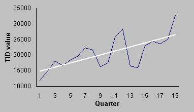
This line graph, below, visually illustrates TID value
versus Quarter number. I have inserted
a trend line that, as you can see, is upward sloping showing that TID increases
over time.
The equation of the
trend line is TID = 14218 + (645.98 * quarter number) with an R2
value of 0.4825.
The trend line might help in predicting future values of
TID, but only predicts 48% of the line chart data.
Average Price versus time
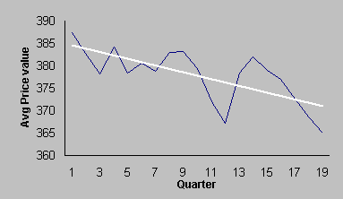
This line graph, below, visually illustrates Average
Price versus Quarter number. I have
inserted a trend line that, as you can see, is downward sloping showing that
Average Price decreases over time.
The equation of the
trend line is Average Price = 385.41 - (0.7625 * quarter number) with an R2
value of 0.4942.
The trend line might help in predicting future Average Prices, but only
predicts 49% of the line chart data.
Average Advertising versus time
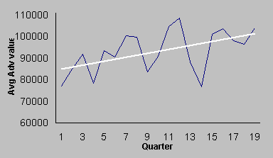
This line graph, below, visually illustrates Average
Advertising dollars spent versus Quarter number. I have inserted a trend line that, as you can see, is upward
sloping showing that Average Advertising increases over time.
The equation of the
trend line is Average Advertising = 84203 + (912.3 * quarter number) with an R2
value of 0.2729.
The trend line might help in predicting future Average Advertising, but
only predicts 27% of the line chart data.
TID versus Average Price
The scatter plot between TID and Average Price (with
an inserted trend line) shows that TID and Average Price have a strong negative
linear relationship (R2 = 0.7898).
TID versus Average Advertising
The scatter plot between TID and Average Advertising
(with an inserted trend line) shows that TID and Average Advertising have a
strong positive linear relationship (R2 = 0.7783); just slightly
weaker than the TID and Average Price relationship.
Average Price versus Average Advertising
The scatter plot between Average Price and Average
Advertising (with an inserted trend line) shows that these two variables
maintain a negative linear relationship.
This one is not as strong as the two above, though: the R2 is
0.5608.
Correlation matrix of TID, Average Price, Average
Advertising, and Quarter
The variables are correlated either
positively or negatively with one another.
In predicting TID, the use of quarter, Average Price, and Average
Advertising may not be necessary as these three variables are correlated with
one another by more than 0.50 each.

RD
Variables:
Here, I
describe RD, PREL, AREL, and RD1.
RD captures relative demand, that is, the demand of EffDee’s product relative
to the demand of products in the industry.
It measures competitive strength.
Relative demand is computed by dividing EffDee’s demand by the average
demand in the industry.
PREL captures relative pricing, that is, the price of EffDee’s product relative
to the price of products in the industry.
It measures competitive and strategic pricing. Relative pricing is computed by dividing EffDee’s price by the
average price in the industry.
AREL captures relative advertising expenditure, that is, EffDee’s amount of
money spent on advertising relative to the amount spent in the industry. It measures promotion of the product. Relative advertising is computed by dividing
EffDee’s amount spent by the average amount spent in the industry.
RD1 captures last quarter’s relative demand; it is a measure of brand
loyalty and is historically recorded.
Relationship of RD with each of PREL, AREL,
and RD1
In the three scatter plots below,
each of the three independent variables is plotted against the dependent variable
RD. From left to right is Relative
Price, Relative Advertising, and Last Quarter’s Relative Demand.
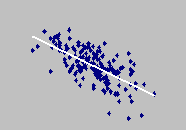
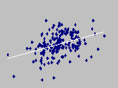
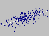
The relationship between Relative
Demand and Relative Price is negative based on the downward sloping trend line
inserted over the scatter plot. As
Relative Price increases, Relative Demand decreases. The trend line equations holds a R2 of 0.4493, that
is, the line can predict 45% of the relationship.
The relationship between Relative
Demand and Relative Advertising is positive based on the upward sloping
trend line inserted over the scatter plot.
As Relative Advertising
increases, Relative Demand also increases. The trend line equations holds a R2 of 0.1431, that
is, the line can predict 14% of the relationship.
The relationship between Relative
Demand and Last Quarter’s Relative Demand is positive based on the upward
sloping trend line inserted over the scatter plot. As Last Quarter’s Relative Demand increases, Relative Demand also
increases. The trend line equations
holds a R2 of 0.505, that is, the line can predict 51% of the
relationship.
For now, it seems
that Relative Price and Relative Advertising are the best predictors of
Relative Demand.
III. Mathematical
Modeling
TID Model
1) Regression analysis using Quarter
(measure of time) as the independent variable to estimate TID
Regression analysis produces the equation:
TID = 14218.07 + (645.98 * Quarter)
R2 =
0.4825
P-value of quarter = 0.00096
2) Regression analysis using Quarter, Average Price, and
Average Advertising as predictors to estimate TID
Regression analysis produces the equation:
TID = 130249.29 + (132.23 * Quarter) – (358.61 * Average
Price) + (0.26 * Average Advertising)
R2 =
0.907
P-value of Quarter = 0.219
P-value of Average Price = 0.010
P-value of Average Advertising = 0.001
3) Regression analysis using Average Price, and Average
Advertising as predictors to estimate TID
Regression analysis produces the equation:
TID = 164336.17 -
(445.17 * Average Price) + (0.26 * Average Advertising)
R2 =
0.897
P-value of Average Price = 0.0006
P-value of Average Advertising = 0.0009
Of the three models above that estimate TID, I believe the
third model is the best. In model 1),
only one variable is used and the R2 value is only 48%. The p-value of this variable is certainly
low (less than 10%), but the R2 value is much lower that model 2)
and 3).
Model 2) gives the best R2 value of the three
models; however, the p-value of Quarter (22%) in this model is over 10%. Model 3) eliminates Quarter as a variable
and returns a R2 value of only one-hundredth of a point lower than
model 2).
RD Model
Regression analysis using PREL, AREL, and
RD1 as predictors of RD
Regression analysis produces the equation:
RD = 16.13 – (16.44 * Relative Price) + (0.78 * Relative
Advertising) + (0.53 * Last Quarter’s Relative Demand)
R2 =
0.958
P-value of Relative Price = 1.0431E-84
P-value of Relative Advertising = 1.33291E-68
P-value of Last Quarter’s Relative Demand = 5.6314E-76
FD Model
The final mathematical model that I can use
to estimate the demand for my product is:
FD = TID * MS =
TID * RD/N
Where,
FD = Firm’s Demand
TID = Total
Industry Demand
MS = Market Share
RD = Relative
Demand
N = Number of
Firms (10)
Expanding this mathematical formula to use the regression formulas from
above used to estimate TID and RD:
FD = [164336.17 - (445.17 * Average Price) + (0.26 * Average
Advertising)] *
[RD = 16.13 – (16.44 * Relative Price) + (0.78 * Relative Advertising)
+ (0.53 * Last Quarter’s Relative Demand)]
/
Number of Firms
Click here to use an
interactive model for predicting Firm’s Demand.